Comparison with Source-Extractor (formerly SExtractor)
Source-Extractor (formerly SExtractor) is a popular astronomical image reduction software that runs in the command line. While both photutils and Source-Extractor serve similar purposes, they do so in subtly different ways and have fundamentally different design principles. Nonetheless, the end-result should be extremely similar, regardless of the choice of software, assuming both are correct.
In this notebook, I compare the results of opticam (photutils-based) to Source-Extractor and show that they are equivalent when configured similarly. For simplicity, image calibrations are omitted from this comparison; instead, opticam’s calibration methods are test in a separate notebook.
A test image
For this example, I’ll use an OPTICAM-MX image of V709 Cas:
[1]:
from pathlib import Path

from astropy.io import fits
import numpy as np

data_path = Path('sextractor_comparison')

data, header = fits.getdata(data_path / 'V709_Cas_image.fits', header=True)
data = np.asarray(data, dtype=np.float64)

print(repr(header))
SIMPLE  =                    T / file does conform to FITS standard
BITPIX  =                   16 / number of bits per data pixel
NAXIS   =                    2 / number of data axes
NAXIS1  =                 1024 / length of data axis 1
NAXIS2  =                 1024 / length of data axis 2
EXTEND  =                    T / FITS dataset may contain extensions
COMMENT   FITS (Flexible Image Transport System) format is defined in 'Astronomy
COMMENT   and Astrophysics', volume 376, page 359; bibcode: 2001A&A...376..359H
BZERO   =                32768 / offset data range to that of unsigned short
BSCALE  =                    1 / default scaling factor
EXPOSURE=                   3. / Single frame exposure time (s)
GAIN    =                   1. / Electronic gain (e-/ADU)
EXPCOAD =                    1 / Number of exposures co-added
CCDTEMP =   -0.439999999999998 / Camera detector temperarure (C)
DETECTOR= 'Andor sCMOS'        / Internal camera name
CCDTYPE = 'Zyla 4.2-P USB 3.0' / Camera Model
SERIALN = 'VSC-05535'          / Camera Serial Number
PIXSIZE =                  6.5 / Pixel Dimensions (in micron)
CCDMODE = '270 MHz '           / Camera Readout Mode
CCDXBIN =                    2 / Binning factor in X
CCDYBIN =                    2 / Binning factor in Y
BINNING = '2x2     '           / Binning [ Cols x Rows ]
DARKCURR=               0.0986 / Dark current (e-/pix/sec)
SATLEVEL=                32302 / Camera saturation level
ORIGIN  = 'UNAM    '           / Origin (Host Institution)
OBSERVAT= 'SPM     '           / Observatory
TELESCOP= '2.1 m   '           / Telescope
INSTRUME= 'OPTICAM '           / Instrument
FOCREDUC= 'f/7.5   '           / Secondary focal reductor
LATITUDE= '+31:02:42'          / Latitude
LONGITUD= '-115:27:58'         / Longitude
ALTITUDE=                 2790 / Altitude
SECONDAR=                   99 / Secondary position(1 step=5um)
TIMEZONE=                    8 / GMT-[N] time zone
OBSERVER= '        '           / Observer name
PROJ_ID = '        '           / Personal project ID
TITLE   = '        '           / Science program title
OBJECT  = 'v709_cas'           / Object
OBS_ID  = 'none    '           / Obs ID
IMGTYPE = 'object  '           / Image type (object/flat/other)
FILTER  = 'g       '           / Filter
FILENAME= '241103g200192105o.fit' / Software-generated filename
ST      = '00:00:00.0000'      / Sideral Time
INITTIME= '2024-11-04 03:46:42.700' / Initial GPS Time
CAM_TIME= '7971988.953600'     / Camera clock Time
UT      = '2024-11-04 05:59:34.688 ' / Universal Time (UT)
UTMIDDLE= '00:00:00.0000'      / UT middle of the observation
RA      = '0:30:14.76'         / Right Ascension
DEC     = '+59:27:15.89'       / Declination
HA      = '-01:29:52.28'       / Hour Angle
AIRMASS =     1.13710990778513 / Airmass
EQUINOX =               2024.8 / Equinox
EPOCH   =                2000. / Epoch (same as Equinox)
JD      =                   0. / Julian Date
DATE-OBS= '2024-11-03'         / Start observation date (UT)
TSTART  =                   0. / Start observation date (UT)
TSTOP   =                   0. / End observation date (UT)
MOONSEP =                   0. / Moon angular separation (deg)
MOONPHAS=                   0. / Moon Phase
AMPNAME = '1 Channel'          / Amplifier name
TMMIRROR=                 99.9 / Primary mirror temperature (C)
TSMIRROR=                 99.9 / Secundary mirror temperature (C)
TAIR    =                 99.9 / Internal telesc air Temp (C)
XTEMP   =                 99.9 / Exterior temperature (C)
HUMIDITY=                 99.9 / External humidity
ATMOSBAR=                 99.9 / Atmosferic presure (in mb)
WIND    = 'XXX at 99.9 km/h'   / Wind direction
WDATE   = '00:00:00, 00/00/00' / Weather acquisition date (UT)
CREATOR = 'MUFFIN  '           / Software application
SOFTVER = '0.9     '           / Software version
AUTHORS = 'A. Castro, E. Colorado & I. Zavala' / Software authors
HISTORY = '        '           / Image history modification log
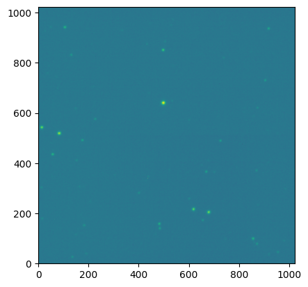
As we can see, this image was taken in the 2x2 binning mode, and so has a resolution of 1024x1024. Let’s take a look at the image:
[2]:
from astropy.visualization import simple_norm
from matplotlib import pyplot as plt

fig, ax = plt.subplots()

ax.imshow(data, origin='lower', norm=simple_norm(data, stretch='log'))

plt.show()
Instead of using opticam.Reducer, since we’re only working with a single image, we’ll compute the image background, identify sources, and perform photometry manually (using opticam’s default values).
By default, opticam uses photutils.segmentation.SourceFinder to perform source detection. This requires specifying an npixels parameter that defines the how many pixels need to be above the specified threshold to constitute a source. opticam defaults to a threshold value of 5. Note: this is the threshold above the background RMS rather than the photometric signal-to-noise ratio. For
npixels, opticam defaults to a value of 128 for images taken in the 1x1 binning mode, and then reduces this value by the square of the image binning. In this case, npixels would therefore be set to \(128/2^2 = 32\):
[3]:
import opticam

threshold = 5

finder = opticam.DefaultFinder(npixels=32)
To compute image backgrounds, opticam uses `photutils.background.Background2D <https://photutils.readthedocs.io/en/stable/user_guide/background.html#d-background-and-noise-estimation>`__. By default, Background2D uses a similar algorithm to Source-Extractor to compute the background. Background2D requires specifying a box_size parameter that determines the size of the background mesh used to compute the two-dimensional background. opticam sets this value to 1/32nd of
the image width; in this case, box_size would therefore be set to \(1024 / 32 = 32\):
[4]:
background = opticam.DefaultBackground(box_size=32)
Let’s compute the background of our image using photutils with opticam’s defaults:
[5]:
bkg = background(data)
data_clean = data - bkg.background
Let’s look at the background subtracted image and the corresponding background mesh to make sure everything looks reasonable:
[6]:
from matplotlib import pyplot as plt

fig, ax = plt.subplots()

im = ax.imshow(data_clean, origin='lower', norm=simple_norm(data_clean, stretch='log'))

bkg.plot_meshes(ax=ax, marker='.', color='red', alpha=.5, outlines=True, markersize=5,)

fig.colorbar(im)

plt.show()
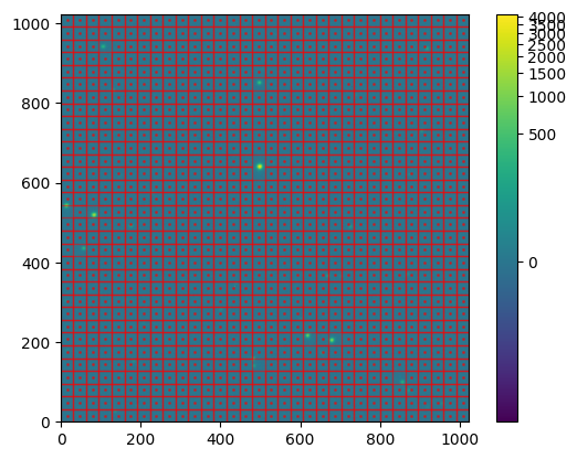
The mesh looks to be a reasonable size: boxes are larger than individual sources while being small enough to capture variations in the background across the image. Let’s now identify the sources in this background-subtracted image:
[7]:
cat = finder(data_clean, 5 * bkg.background_rms)

cat.pprint_all()
label     xcentroid          ycentroid      sky_centroid bbox_xmin bbox_xmax bbox_ymin bbox_ymax  area  semimajor_sigma    semiminor_sigma      orientation         eccentricity        min_value          max_value      local_background    segment_flux    segment_fluxerr     kron_flux      kron_fluxerr
                                                                                                  pix2        pix                pix                deg
----- ------------------ ------------------ ------------ --------- --------- --------- --------- ----- ------------------ ------------------ ------------------ ------------------- ------------------ ------------------ ---------------- ------------------ --------------- ------------------ ------------
   17  497.6804172508962  638.9789666325404         None       487       509       627       650 388.0 3.3659313208722703 3.2560953687948078  37.82102520710939 0.25337424789937224  40.59610558563881 3822.5553110448236              0.0  217086.6513927103             nan 217848.78308915766          nan
   14  82.96791080424372  517.7716881918581         None        74        92       509       527 270.0  3.221563164883371  3.062450948908997 18.673396074349174 0.31038711703603666   40.6866877157088 1640.7586194772389              0.0  95878.79741579312             nan  98622.72229736176          nan
    8  678.1251572633767 203.64531890802692         None       670       687       196       211 222.0   3.10171672006387 2.8973018951612843  48.03943502089947 0.35702133388051005  41.00075222595538 1210.8611411097218              0.0  60759.33118800631             nan  64257.11170117938          nan
   15 13.734081255269217  541.3878040504604         None         6        23       533       549 199.0  3.056615529101678  2.839502657399498 22.688464924897215 0.37015622787568264  41.00184523402491  1005.020688400301              0.0  52526.58026598147             nan  56010.03740272815          nan
    9   617.696069097033 215.47627042751554         None       609       626       207       224 196.0 3.0437434358950033  2.815631467704122  63.86621527373709  0.3798320760013057 41.371333294861174  906.3671147884698              0.0  43758.14814852801             nan  47165.57676704407          nan
   20 496.73461387402585  849.5099247452262         None       490       504       842       855 141.0 2.7499477590867403  2.528166820765207  13.51959389176717 0.39343869567426404  40.16573833079882  574.1699468123657              0.0  23633.70800168105             nan  27134.47662940775          nan
   22  105.8291616121421  940.2001346853478         None       100       113       934       946 121.0 2.7511807051764867 2.4490379537260702 16.723014561911377  0.4556147501064043  40.64326094193774   305.616318524162              0.0 15235.622433186916             nan 18523.229370860077          nan
    3  855.0108482904118  98.39239267318543         None       849       861        92       104 115.0 2.6090568267271474  2.552554802018481 51.722241588913654 0.20698607490397405  40.31347212879321  304.4766470218045              0.0 13752.749367060878             nan 16884.047076496747          nan
   11  57.24792217829644  434.2802011682957         None        51        63       429       440 109.0 2.5378868918225552 2.4073698239892978   -6.0737060151497 0.31655983604097365  40.92290451240622 319.02927765258187              0.0 13672.099928960126             nan 16966.737370715982          nan
    6 481.55431956049455 157.19113596313497         None       475       487       150       163 103.0  2.631629222791232  2.320658827531296  81.86309992543326  0.4715608819087923  40.77294762276678 314.80873872419795              0.0 12297.790396497785             nan 15663.551998404795          nan
   21  916.6923291357015  935.0932198100281         None       912       921       930       940  77.0 2.3301381354883173 2.1145977428687104 46.883802725728515  0.4200545047397276  39.73289364433387  224.7014714117856              0.0  7614.922895066142             nan 10749.284422262735          nan
   13 175.28479635184814  490.5600173840552         None       170       181       486       495  73.0  2.446317626046904 1.9771668217777325  4.288230770607925  0.5888784213324333 39.571712999041864 159.60203459854057              0.0   6272.15087812934             nan   8808.58922230818          nan
   10   668.692646486444  365.0946676837512         None       664       673       360       369  68.0 2.3370094207711127 1.9881466348278292 53.384591914528556  0.5256149994257804  40.39597855723848  163.4028983733722              0.0  5752.257748138215             nan   8120.04065963446          nan
    4 483.35923216903683 139.55454018014115         None       479       488       134       144  67.0 2.2158132266829846 2.0249732733799055  70.60038063853762  0.4059987577199394   40.8405912857897  174.8580294541618              0.0  5449.884823311359             nan  8666.641184434746          nan
   12  724.9659552048159  488.1684109068366         None       720       729       484       493  63.0 2.1715650556309374  2.022401697509871  24.08092674613499  0.3642258145785818 39.511669972988884 122.59461389965243              0.0  4537.207173863786             nan  6386.483726610832          nan
   18  903.3840355342294  729.0736854720369         None       899       908       726       734  52.0  1.925000530363993 1.8676042681920093 -7.648612810365687 0.24237049338960892  40.22571937016528 153.20556634365053              0.0 3850.7003654749765             nan  6160.585775591036          nan
   19  131.5501905141806  830.0797530149874         None       128       136       826       835  51.0  2.010969803660195 1.8769995766192156 -28.83056823253136 0.35888889089169906  39.94124123924051  119.9469647496916              0.0  3475.413489189245             nan  5916.584806355414          nan
    2   870.308814876515  77.87491727677332         None       866       874        74        82  46.0 2.1477237512426957 1.7129036712989125  48.63710589494355   0.603261099675754  41.55049608260023 130.80561087260045              0.0 3356.7723548046747             nan  6832.660078301629          nan
   16 226.32362665027642  574.9788224800949         None       222       231       571       578  42.0 2.4280297686052985 1.6552704750614462 27.970962965533456  0.7316001210198605  39.29192658530623 174.23964940240495              0.0  2791.533186641267             nan 5377.6502602056935          nan
    7   654.426908239823 171.86640296658106         None       651       658       169       175  34.0  1.838554382718119 1.5857441614988306 37.528291665421314  0.5060653990359425  43.59568000935269  97.61473407246856              0.0  2199.672576344242             nan  4363.760027899712          nan
    5 182.33594341117333  151.5531715207304         None       179       186       148       154  35.0 1.9613937197826732 1.5821389935348982  57.27844554773467  0.5910428169680217 41.369632087967815 123.34543397865811              0.0 2186.7947048985816             nan 4978.3085885298005          nan
    1  135.8775804601037 25.520119715310464         None       133       139        21        29  37.0  2.104203313802178 1.4946217779675977  74.29332747907334  0.7038961204640036  41.39635247491037   85.3911817848913              0.0 2127.7688145727293             nan   4016.95432804196          nan
As we can see, a number of sources have been identified (22, to be specific). Let’s take a look at these sources:
[8]:
import numpy as np

source_coords = np.asarray([cat['xcentroid'], cat['ycentroid']]).T

semimajor_sigma = np.median(cat['semimajor_sigma'].value)
radius = 5 * semimajor_sigma  # aperture radius for plotting
[9]:
from matplotlib import pyplot as plt
from matplotlib.patches import Circle

fig, ax = plt.subplots()

im = ax.imshow(data_clean, origin='lower', norm=simple_norm(data_clean, stretch='log'))

for coords in source_coords:
    ax.add_patch(
        Circle(coords, radius=radius, edgecolor='red', facecolor='none')
    )

fig.colorbar(im)

plt.show()
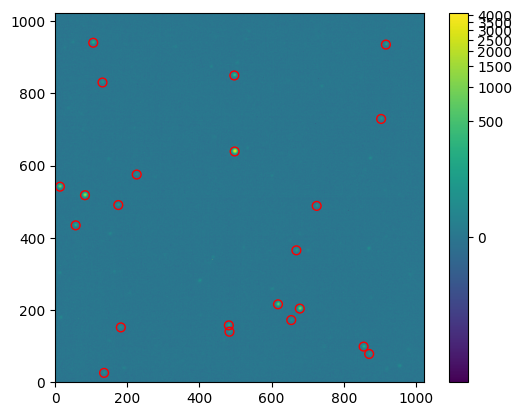
Source detection looks reasonable. Let’s move on to photometry.
For comparison with Source-Extractor, we’ll only look at aperture photometry. To perform aperture photometry, opticam uses the `photutils.aperture <https://photutils.readthedocs.io/en/stable/user_guide/aperture.html>`__ subpackage. This subpackage defines convenience routines for defining apertures and performing aperture photometry. For simplicity, we’ll use a circular aperture with a 5 pixel radius. By default, opticam defines an
`EllipticalAperture <https://photutils.readthedocs.io/en/stable/api/photutils.aperture.EllipticalAperture.html#photutils.aperture.EllipticalAperture>`__, so we’ll make it circular by passing the same value to both axes, and setting the orientation of the ellipse to 0 degrees:
[10]:
photometer = opticam.AperturePhotometer(
    semimajor_axis=5,
    semiminor_axis=5,
    orientation=0.,
    forced=True,  # use forced photometry since we only have one image
    )

results = photometer.compute(
    image=data_clean,
    bias_var=0.,  # ignore bias variance
    dark_var=0.,  # ignore dark variance
    flat_var=0.,  # ignore flat variance
    background_rms=bkg.background_rms,
    cat_coords=source_coords,
    image_coords=None,  # not needed since forced=True
    psf_params=None,  # not needed since aperture size set manually
    read_noise=0.,  # ignore read noise
    )

fluxes = np.asarray(results['flux'])
flux_errs = np.asarray(results['flux_err'])
One important difference between opticam/photutils and Source-Extractor is how apertures handle partially overlapping pixels. By default, photutils (and, by extension, opticam) computes the exact fractional overlap of each pixel with the aperture. In contrast, Source-Extractor divides pixels into 5x5 subpixels, and includes subpixels whose centres fall within the aperture.
photutils can be configured to perform the same subpixelling as Source-Extractor, but this is not the default behaviour. As such, opticam will generally result in slightly different flux values when compared to Source-Extractor.
Source-Extractor
To run Source-Extractor, a number of configuration files are required. We therefore need to tweak these configuration files to match the default behaviour of opticam. In particular, we need to edit default.sex to set DETECT_MINAREA to 32, DETECT_THRESH and ANALYSIS_THRESH to 5, PHOT_APERTURES to 10 (since this quantifies the diameter of the aperture), and BACK_SIZE (background mesh size) to 32. The full configuration file used is given below:
[11]:
with open(data_path / 'opticam_default.sex', 'r') as file:
    print(file.read())
# Default configuration file for SExtractor V1.2b14 - > 2.0
# EB 23/07/98
# (*) indicates parameters which can be omitted from this config file.

#-------------------------------- Catalog ------------------------------------

CATALOG_NAME    test.cat        # name of the output catalog
CATALOG_TYPE    FITS_1.0        # "NONE","ASCII_HEAD","ASCII","FITS_1.0" or "FITS_LDAC"

PARAMETERS_NAME opticam_default.param   # name of the file containing catalog contents

#------------------------------- Extraction ----------------------------------

DETECT_TYPE     CCD             # "CCD" or "PHOTO" (*)
FLAG_IMAGE      flag.fits       # filename for an input FLAG-image
DETECT_MINAREA  32              # minimum number of pixels above threshold

THRESH_TYPE     RELATIVE        # threshold type: RELATIVE (in sigmas)
DETECT_THRESH   5               # <sigmas>
ANALYSIS_THRESH 5               # <sigmas>

FILTER          N               # apply filter for detection ("Y" or "N")?
FILTER_NAME     default.conv    # name of the file containing the filter

DEBLEND_NTHRESH 32              # Number of deblending sub-thresholds
DEBLEND_MINCONT 0.1             # Minimum contrast parameter for deblending

CLEAN           N               # Clean spurious detections? (Y or N)?
CLEAN_PARAM     1.0             # Cleaning efficiency

MASK_TYPE       CORRECT         # type of detection MASKing: can be one of "NONE", "BLANK" or "CORRECT"

#------------------------------ Photometry -----------------------------------


PHOT_APERTURES  10              # MAG_APER aperture diameter(s) in pixels
PHOT_AUTOPARAMS 2.5,3.5         # MAG_AUTO parameters: <Kron_fact>,<min_radius>

SATUR_LEVEL     65535.0         # level (in ADUs) at which arises saturation

MAG_ZEROPOINT   0.0             # magnitude zero-point
MAG_GAMMA       4.0             # gamma of emulsion (for photographic scans)
GAIN            1.0             # detector gain in e-/ADU.
PIXEL_SCALE     1.0             # size of pixel in arcsec (0=use FITS WCS info).

#------------------------- Star/Galaxy Separation ----------------------------

SEEING_FWHM     1.2             # stellar FWHM in arcsec
STARNNW_NAME    default.nnw     # Neural-Network_Weight table filename

#------------------------------ Background -----------------------------------

BACK_SIZE       32              # Background mesh: <size> or <width>,<height>
BACK_FILTERSIZE 3               # Background filter: <size> or <width>,<height>

BACKPHOTO_TYPE  GLOBAL          # can be "GLOBAL" or "LOCAL" (*)
BACKPHOTO_THICK 24              # thickness of the background LOCAL annulus (*)

#------------------------------ Check Image ----------------------------------

#CHECKIMAGE_TYPE        BACKGROUND,BACKGROUND_RMS,-BACKGROUND,FILTERED,OBJECTS,APERTURES,SEGMENTATION

#CHECKIMAGE_NAME        check_bkg.fits,check_bkg_RMS.fits,check_-bkg.fits,check_filt.fits,check_obj.fits,check_ap.fits,check_segm.fits  # Filename for the check-image (*)

#--------------------- Memory (change with caution!) -------------------------

MEMORY_OBJSTACK 2000            # number of objects in stack
MEMORY_PIXSTACK 100000          # number of pixels in stack
MEMORY_BUFSIZE  1024            # number of lines in buffer

#----------------------------- Miscellaneous ---------------------------------

VERBOSE_TYPE    NORMAL          # can be "QUIET", "NORMAL" or "FULL" (*)

#------------------------------- New Stuff -----------------------------------
I also edited the default.param configuration file to only save the following columns in the resulting catalogue:
[12]:
with open(data_path / 'opticam_default.param', 'r') as file:
    print(file.read())
NUMBER
X_IMAGE
Y_IMAGE
FLUX_APER
FLUXERR_APER
Source-Extractor is a command line tool, so it’s not as easy as photutils to run it in a notebook like this. However, we can use the `os.system() <https://docs.python.org/3/library/os.html#os.system>`__ function to pass the required commands to the system shell:
[13]:
import os

image_path = data_path.joinpath('V709_Cas_image.fits').resolve()
os.chdir(os.path.join(os.getcwd(), 'sextractor_comparison'))
os.system(f'source-extractor {image_path} -c opticam_default.sex')
os.chdir(os.path.join(os.getcwd(), '..'))  # go back to original directory
>
----- Source Extractor 2.28.0 started on 2026-02-16 at 18:32:44 with 1 thread

> Setting catalog parameters
> Initializing catalog
> Looking for V709_Cas_image.fits
----- Measuring from: V709_Cas_image.fits
      "v709_cas" / no ext. header / 1024x1024 / 16 bits (integers)
Detection+Measurement image: > Setting up background maps
> Filtering background map(s)
> Computing background d-map
> Computing background-noise d-map
(M+D) Background: 117.514    RMS: 7.8876     / Threshold: 39.438
> Scanning image
> Line:   25  Objects:        0 detected /        0 sextracted
> Line:   50  Objects:        1 detected /        0 sextracted
> Line:   75  Objects:        1 detected /        0 sextracted
> Line:  100  Objects:        2 detected /        0 sextracted
> Line:  125  Objects:        3 detected /        0 sextracted
> Line:  150  Objects:        4 detected /        0 sextracted
> Line:  175  Objects:        6 detected /        0 sextracted
> Line:  200  Objects:        7 detected /        0 sextracted
> Line:  225  Objects:        8 detected /        0 sextracted
> Line:  250  Objects:        9 detected /        0 sextracted
> Line:  275  Objects:        9 detected /        0 sextracted
> Line:  300  Objects:        9 detected /        0 sextracted
> Line:  325  Objects:        9 detected /        0 sextracted
> Line:  350  Objects:        9 detected /        0 sextracted
> Line:  375  Objects:       10 detected /        0 sextracted
> Line:  400  Objects:       10 detected /        0 sextracted
> Line:  425  Objects:       10 detected /        0 sextracted
> Line:  450  Objects:       11 detected /        0 sextracted
> Line:  475  Objects:       11 detected /        0 sextracted
> Line:  500  Objects:       13 detected /        0 sextracted
> Line:  525  Objects:       13 detected /        0 sextracted
> Line:  550  Objects:       14 detected /        0 sextracted
> Line:  575  Objects:       15 detected /        0 sextracted
> Line:  600  Objects:       16 detected /        0 sextracted
> Line:  625  Objects:       16 detected /        0 sextracted
> Line:  650  Objects:       16 detected /        0 sextracted
> Line:  675  Objects:       17 detected /        0 sextracted
> Line:  700  Objects:       17 detected /        0 sextracted
> Line:  725  Objects:       17 detected /        0 sextracted
> Line:  750  Objects:       18 detected /        0 sextracted
> Line:  775  Objects:       18 detected /        0 sextracted
> Line:  800  Objects:       18 detected /        0 sextracted
> Line:  825  Objects:       18 detected /        0 sextracted
> Line:  850  Objects:       19 detected /        0 sextracted
> Line:  875  Objects:       20 detected /        0 sextracted
> Line:  900  Objects:       20 detected /        0 sextracted
> Line:  925  Objects:       20 detected /        0 sextracted
> Line:  950  Objects:       22 detected /        0 sextracted
> Line:  975  Objects:       22 detected /        0 sextracted
> Line: 1000  Objects:       22 detected /        0 sextracted
> Line: 1024  Objects:       22 detected /        0 sextracted
> Line: 1024  Objects:       22 detected /        1 sextracted
      Objects: detected 22       / sextracted 22

> Closing files
>
> All done (in 0.0 s: 72341.2 lines/s , 1554.2 detections/s)
We can see that 22 sources were detected, just like photutils. We can also see that the image background was 117.514 with an RMS of 7.8876. Let’s compare these values to those computed by photutils:
[14]:
print(round(bkg.background_median, 3), round(bkg.background_rms_median, 4))
117.535 7.8861
The background values are extremely similar, as we would hope. Slight differences are likely due to different sigma clipping parameters. Source-Exractor will iteratively clip pixels within a mesh box until all pixels are within :math:`3 sigma of the median value <https://sextractor.readthedocs.io/en/latest/Background.html#background-estimation>`__. By default, photutils (and, by extension, opticam) uses the same sigma clipping threshold, but only performs up to 10
iterations. Since photutils uses an `astropy.stats.SigmaClip <https://docs.astropy.org/en/stable/api/astropy.stats.SigmaClip.html#astropy.stats.SigmaClip>`__ instance to perform sigma clipping, it can be configured to clip until convergence is acheived, as in Source-Extractor, by defining a SigmaClip instance with maxiters=None. However, this is not the default
behaviour. As such, opticam will generally result in slightly different background values when compared to Source-Extractor.
Let’s now take a look at the resulting catalogue:
[15]:
from astropy.table import Table

sextractor_cat = Table.read(data_path / 'test.cat', format="fits")
sextractor_cat.sort('FLUX_APER', reverse=True)

sextractor_cat.pprint()
  NUMBER     X_IMAGE     Y_IMAGE    FLUX_APER   FLUXERR_APER
               pix         pix          ct           ct
---------- ----------- ----------- ------------ ------------
         7    498.6823    639.9772     151779.8     395.8028
        10     83.9666    518.7689     68195.27     270.3383
        16    679.1282    204.6347     44607.61     222.4695
         9     14.7341    542.3884     38965.54     209.3935
        15    618.7043    216.4675      32732.8     194.0046
         4    497.7347    850.5096     19265.88     155.4618
         2    106.8367    941.2122     12632.92     132.3461
        13     58.2004    435.2825     11839.58     129.2564
        21    856.0100     99.3910     11569.81     128.2183
       ...         ...         ...          ...          ...
        14    669.6926    366.0947     5938.621     104.1445
        20    484.3595    140.5544     5709.391     102.9777
        12    725.9660    489.1685     4928.967     99.07835
         6    904.3840    730.0735     4524.715     97.00402
         5    132.5502    831.0798     4217.494     95.42037
        22    871.3052     78.8281     4209.681     95.30112
         8    227.3283    576.0359     3578.154     91.98223
        19    183.3837    152.5432     3187.841     89.82165
        17    655.4283    172.8654     3163.659     89.70081
         1    136.9534     26.4141     3153.166     89.67006
Length = 22 rows
We can see that we have the coordinates of each detected source as well as the measured flux values and their corresponding errors. Let’s see how the detected sources compare to those of photutils:
[16]:
from matplotlib.patches import Rectangle

sextractor_coords = np.asarray([sextractor_cat['X_IMAGE'], sextractor_cat['Y_IMAGE']]).T

fig, ax = plt.subplots()

ax.imshow(data_clean, origin='lower', norm=simple_norm(data_clean, stretch='log'))

for coords in source_coords:
    ax.add_patch(
        Circle(coords, radius=radius, edgecolor='red', facecolor='none')
    )

for coords in sextractor_coords:
    ax.add_patch(
        Rectangle(coords - radius, width=2 * radius, height= 2 * radius, edgecolor='white', facecolor='none', zorder=0)
    )

plt.show()
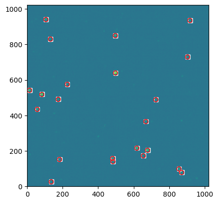
As we can see, source identification appears identical.
Let’s now compare the measured fluxes:
[17]:
sextractor_fluxes = np.asarray(sextractor_cat['FLUX_APER'])
sextractor_flux_errs = np.asarray(sextractor_cat['FLUXERR_APER'])

fig, ax = plt.subplots()

ax.plot(sextractor_fluxes, sextractor_flux_errs, 'r+', label='Source-Extractor')
ax.plot(fluxes, flux_errs, 'kx', label='opticam')

ax.set_xscale('log')
ax.legend(fontsize='large')

ax.set_ylabel('Flux error [ADU]', fontsize='large')
ax.set_xlabel('Flux [ADU]', fontsize='large')
ax.minorticks_on()
ax.tick_params(which='both', direction='in', right=True, top=True)

plt.show()
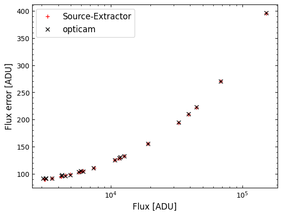
Reassuringly, there looks to be very little difference between the two programs. Let’s compare the results more quantitatively.
[18]:
err_ratio = flux_errs / sextractor_flux_errs
print(f'Average error ratio: {err_ratio.mean()}')
print(f'Max err ratio: {err_ratio.max()}')
print(f'Max err ratio: {err_ratio.min()}')
print()

ratio = fluxes / sextractor_fluxes
print(f'Average ratio: {ratio.mean()}')
print(f'Max ratio: {ratio.max()}')
print(f'Min ratio: {ratio.min()}')
Average error ratio: 1.005002830885876
Max err ratio: 1.0260424921219515
Max err ratio: 0.9893920036519251

Average ratio: 1.0009324631316407
Max ratio: 1.0257912595904741
Min ratio: 0.9766904198791279
As we can see, opticam (using photutils) performs very similarly to Source-Extractor when both are configured similarly. On average, the difference between opticam/photutils and Source-Extractor was less than 1% in this example, with extremes of \(\sim 2.5\)%. As noted above, this difference is due to a combination of how opticam and Source-Extractor treat partially overlapping pixels differently, and use different sigma clipping parameters.
[19]:
assert np.isclose(err_ratio.mean(), 1., rtol=0.01, atol=0.)
assert np.isclose(ratio.mean(), 1., rtol=0.01, atol=0.)
That concludes this comparison between opticam and Source-Extractor.