Identifying sources

opticam_new uses photutils to find sources in images. This notebook will demonstrate how to define source finders for use with opticam_new, as well as explain opticam_new’s default behaviour when no source finder is specified.

Test Image

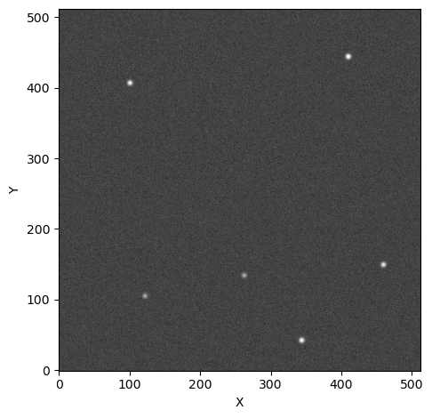
First thing’s first, let’s open an image that contains some sources. For this example, I’ll use one of the images from the Basic Usage tutorial:

import opticam_new

opticam_new.generate_observations(
    out_dir='finders_tutorial/data',
    n_images=20,
    circular_aperture=False,
    )

[OPTICAM] variable source is at (122, 104)

Generating observations: 100%|██████████|[00:04<00:00]

from astropy.io import fits
import numpy as np
import os

files = os.listdir("finders_tutorial/data")
file = files[0]

with fits.open(f"finders_tutorial/data/{file}") as hdul:
    print(repr(hdul[0].header))
    image = np.array(hdul[0].data)
    binning_factor = int(hdul[0].header['BINNING'][0])

SIMPLE  =                    T / conforms to FITS standard
BITPIX  =                  -64 / array data type
NAXIS   =                    2 / number of array dimensions
NAXIS1  =                  512
NAXIS2  =                  512
EXTEND  =                    T
FILTER  = 'i       '
BINNING = '4x4     '
GAIN    =                  1.0
UT      = '2024-01-01 00:00:12'

from astropy.visualization import simple_norm
from matplotlib import pyplot as plt

fig, ax = plt.subplots(tight_layout=True)

im = ax.imshow(image, norm=simple_norm(image, stretch="sqrt"), origin="lower", cmap="Greys_r")

ax.set_xlabel("X")
ax.set_ylabel("Y")

plt.show()

Default Finder

opticam_new implements two default source finders: Finder (default) and CrowdedFinder (better for crowded fields, but more expensive). Finder does not implement any source deblending, while CrowdedFinder does. Both of these source finders are wrappers for photutils.segmentation.SourceFinder with some added convenience tailored to OPTICAM.

Let’s use opticam_new.Finder to identify the sources in the above image:

from opticam_new import DefaultFinder

from photutils.segmentation import detect_threshold

# default value for npixels is 128 // binning_factor**2
# default value for border_width is 1/16th of the image width
default_finder = DefaultFinder(npixels=128 // 4**2, border_width=image.shape[0] // 16)

default_segm = default_finder(image, threshold=detect_threshold(image, nsigma=5))  # detect sources above 5 sigma
print(type(default_segm))

<class 'photutils.segmentation.core.SegmentationImage'>

When calling a DefaultFinder() instance, a `SegmentationImage <https://photutils.readthedocs.io/en/stable/user_guide/segmentation.html>`__ is returned. This can be used to define a SourceCatalog:

from photutils.segmentation import SourceCatalog

tbl = SourceCatalog(data=image, segment_img=default_segm).to_table()

print(tbl)

label     xcentroid          ycentroid      ...     kron_flux     kron_fluxerr
                                            ...
----- ------------------ ------------------ ... ----------------- ------------
    1 343.50869723873694 42.920775668063335 ... 97240.28273022271          nan
    2 121.71262540499553  105.5502562842776 ...  84251.0093768113          nan
    3 262.07427576900153 134.55645675772124 ... 81260.76519898814          nan
    4  459.1601803809478  149.7953651395983 ... 94897.71701537866          nan
    5 100.36621469873283 406.86369869058916 ... 92466.82927165771          nan
    6  409.5092033513822  444.2089681224758 ... 98622.62071081837          nan

This is how catalogs are defined in opticam_new. We can also plot the SegmentationImage directly to see the sources:

fig, axs = plt.subplots(ncols=2, tight_layout=True, figsize=(10, 5))

axs[0].set_title("Original")
axs[0].imshow(image, norm=simple_norm(image, stretch="sqrt"), origin="lower", cmap="Greys_r", interpolation='nearest')

axs[1].set_title("Segmentation Map")
axs[1].imshow(default_segm, origin="lower", cmap=default_segm.cmap, interpolation="nearest")

plt.show()

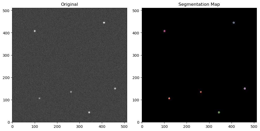
As we can see, all the sources have been correctly identified.

Custom Source Finders

Defining the Source Finder

Let’s now define a custom source finder. Custom source finders must define a __call__() method that takes two parameters: image and threshold, and returns a SegmentationImage. image should be an NDArray containing the image data. threshold defines the threshold for source detection, typically defined in units of the background RMS:

from photutils.segmentation import SourceFinder

class CustomFinder:

    def __init__(self, border_width = 0, **kwargs):

        self.border_width = border_width

        self.finder = SourceFinder(**kwargs)

    def __call__(self, image, threshold):

        segment_map = self.finder(image, threshold)
        segment_map.remove_border_labels(border_width=self.border_width, relabel=True)

        return segment_map

This source finder is basically a wrapper for the SourceFinder class from photutils with an additional border_width parameter. It implements a custom __call__() method that identifies sources and removes source labels close to the edge of the image, just like opticam_new.DefaultFinder. Let’s initialise this custom source finder and use it to identify sources in the above image. We’ll set the npixels and border_width parameters to the same values assumed by opticam_new.DefaultFinder, but set some custom values for the other parameters:

custom_finder = CustomFinder(npixels=128 // 4**2, border_width=image.shape[0] // 16, deblend=True,
                             nlevels=256, contrast=0, progress_bar=False)

custom_segm = custom_finder(image, threshold=detect_threshold(image, nsigma=5))

Let’s plot the image to see what it looks like:

fig, axs = plt.subplots(ncols=2, tight_layout=True, figsize=(10, 5))

axs[0].set_title("Original")
axs[0].imshow(image, norm=simple_norm(image, stretch="sqrt"), origin="lower", cmap="Greys_r", interpolation='nearest')

axs[1].set_title("Segmentation Map")
axs[1].imshow(custom_segm, origin="lower", cmap=custom_segm.cmap, interpolation="nearest")

plt.show()

As we can see, we have once again recovered all six sources. We could also pass our custom source finder to opticam_new.Catalog:

cat = opticam_new.Catalog(
    out_directory='finders_tutorial/results',
    data_directory='finders_tutorial/data',
    finder=custom_finder,
    remove_cosmic_rays=False,
)

[OPTICAM] finders_tutorial/results not found, attempting to create ...
[OPTICAM] finders_tutorial/results created.

[OPTICAM] Scanning data directory: 100%|██████████|[00:00<00:00]

[OPTICAM] Binning: 4x4
[OPTICAM] Filters: g-band, r-band, i-band
[OPTICAM] 20 g-band images.
[OPTICAM] 20 r-band images.
[OPTICAM] 20 i-band images.

cat.create_catalogs()

[OPTICAM] Initialising catalogs

[OPTICAM] Aligning g-band images: 100%|██████████|[00:00<00:00]

[OPTICAM] Done.
[OPTICAM] 20 image(s) aligned.
[OPTICAM] 0 image(s) could not be aligned.

[OPTICAM] Aligning r-band images: 100%|██████████|[00:00<00:00]

[OPTICAM] Done.
[OPTICAM] 20 image(s) aligned.
[OPTICAM] 0 image(s) could not be aligned.

[OPTICAM] Aligning i-band images: 100%|██████████|[00:00<00:00]

[OPTICAM] Done.
[OPTICAM] 20 image(s) aligned.
[OPTICAM] 0 image(s) could not be aligned.

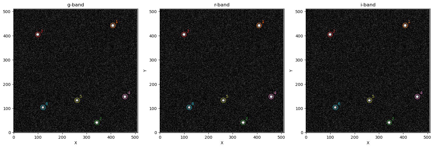
Once again, we have successfully identified all six sources. Admittedly, this rather simple example does a poor job of demonstrating why defining a custom source finder may be useful, but hopefully it is clear how custom source finders can be implemented. For more information on defining custom source finders, I refer to the excellent photutils documentation: https://photutils.readthedocs.io/en/stable/user_guide/segmentation.html.

That concludes the source finder tutorial for opticam_new!