Identifying sources
opticam uses photutils to find sources in images. This notebook will demonstrate how to define source finders for use with opticam, as well as explain opticam’s default behaviour when no source finder is specified.
Test Image
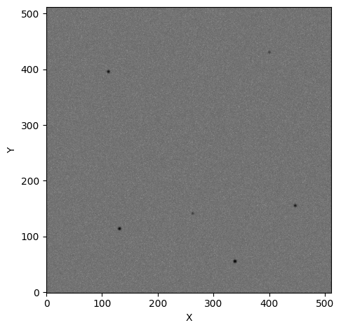
First thing’s first, let’s open an image that contains some sources. For this example, I’ll use one of the images from the Basic Usage tutorial:
[1]:
import opticam

opticam.generate_observations(
    out_dir='finders_tutorial/data',
    n_images=3,
    circular_aperture=False,
    )
[OPTICAM] variable source is at (131, 115)
[OPTICAM] variability RMS: 0.02 %
[OPTICAM] variability frequency: 0.135 Hz
[OPTICAM] variability phase lags:
    [OPTICAM] g-band: 0.000 radians
    [OPTICAM] r-band: 1.571 radians
    [OPTICAM] i-band: 3.142 radians
Generating observations: 100%|██████████|[00:01<00:00]
[2]:
from astropy.io import fits
import numpy as np
import os

files = os.listdir("finders_tutorial/data")
file = files[0]

with fits.open(f"finders_tutorial/data/{file}") as hdul:
    print(repr(hdul[0].header))
    image = np.array(hdul[0].data)
    binning_factor = int(hdul[0].header['BINNING'][0])
SIMPLE  =                    T / conforms to FITS standard
BITPIX  =                  -64 / array data type
NAXIS   =                    2 / number of array dimensions
NAXIS1  =                  512
NAXIS2  =                  512
EXTEND  =                    T
FILTER  = 'i       '
BINNING = '4x4     '
GAIN    =                  1.0
EXPOSURE=                  1.0
DARKCURR=                  0.0
RA      =                  0.0
DEC     =                  0.0
UT      = '2024-01-01 00:00:00'
[3]:
from astropy.visualization import simple_norm
from matplotlib import pyplot as plt

fig, ax = plt.subplots(tight_layout=True)

im = ax.imshow(
    image,
    norm=simple_norm(image, stretch="log"),
    origin="lower",
    cmap="Greys",
    )

ax.set_xlabel("X")
ax.set_ylabel("Y")

plt.show()
Default Finder
opticam implements two default source finders: Finder (default) and CrowdedFinder (better for crowded fields, but more expensive). Finder does not implement any source deblending, while CrowdedFinder does. Both of these source finders are wrappers for photutils.segmentation.SourceFinder with some added convenience tailored to OPTICAM.
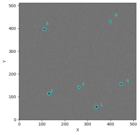
Let’s use opticam.Finder to identify the sources in the above image:
[4]:
from opticam import DefaultFinder

from photutils.segmentation import detect_threshold

# default value for npixels is 128 // binning_factor**2
# default value for border_width is 1/16th of the image width
default_finder = DefaultFinder(npixels=128 // 4**2, border_width=image.shape[0] // 16)

default_tbl = default_finder(
    image,
    threshold=detect_threshold(image, nsigma=5),  # 5 sigma detection threshold
    )
print(type(default_tbl))
<class 'astropy.table.table.QTable'>
When calling a DefaultFinder() instance, an astropy.table.QTable instance is returned that is sorted in descending order of source flux. This is how catalogs are defined in opticam. We can use the table to visualise which sources have been identified and how their fluxes are ranked:
[5]:
from matplotlib.patches import Circle

fig, ax = plt.subplots(
    tight_layout=True,
    )

im = ax.imshow(
    image,
    norm=simple_norm(image, stretch="log"),
    origin="lower",
    cmap="Greys",
    )

for i, row in enumerate(default_tbl):

    xc = row['xcentroid']
    yc = row['ycentroid']

    ax.add_patch(
        Circle(
            xy=(xc, yc),
            radius=5 * row['semimajor_sigma'].value,
            facecolor='none',
            edgecolor='cyan',
            lw=1,
        )
    )

    ax.text(
        xc * 1.05,
        yc * 1.05,
        f'{i + 1}',
        color='cyan',
    )

ax.set_xlabel("X")
ax.set_ylabel("Y")

plt.show()
Custom Source Finders
Defining the Source Finder
Let’s now define a custom source finder. A custom source finder must be a callable that takes two parameters: image and threshold, and returns a QTable instance. image should be an NDArray containing the image data. threshold defines the threshold for source detection in ADU. The simplest way to define a custom source finder is by using the photutils.segmentation.SourceFinder class, which combines source detection and deblending:
[6]:
from photutils.segmentation import SourceCatalog, SourceFinder

def custom_finder(image, threshold):
    finder = SourceFinder(
        npixels=128 // 4**2,  # same as DefaultFinder
        deblend=True,  # same as DefaultFinder
        nlevels=256,  # higher than DefaultFinder (more deblending)
        contrast=0,  # higher than DefaultFinder (more deblending)
        progress_bar=False,  # disable progress bar (same as DefaultFinder)
        )
    segment_img = finder(image, threshold)

    tbl = SourceCatalog(image, segment_img).to_table()
    tbl.sort('segment_flux', reverse=True)  # sort in descending order

    return tbl
Under-the-hood, opticam.DefaultFinder also uses photutils.segmentation.SourceFinder, but here we have defined our custom source finder to use different parameter values for better source deblending (though deblending isn’t really needed for our example images). In addition to the different parameter values, our custom finder differs from DefaultFinder in that DefaultFinder automatically omits sources that are close to the edge of an image (where “close” is defined as 1/16th of
the image width, the same size as the default background pixels). For this example, this will not make a difference but it can be important in practise. To understand how to remove sources from a SegmentationImage that are too close to an edge, I refer to the excellent photutils documentation: https://photutils.readthedocs.io/en/stable/user_guide/segmentation.html.
Let’s now initialise this custom source finder and use it to identify sources in the above image.
[7]:
custom_tbl = custom_finder(
    image,
    threshold=detect_threshold(image, nsigma=5),  # 5 sigma detection threshold
    )
[8]:
fig, ax = plt.subplots(
    tight_layout=True,
    )

im = ax.imshow(
    image,
    norm=simple_norm(image, stretch="log"),
    origin="lower",
    cmap="Greys",
    )

for i, row in enumerate(custom_tbl):

    xc = row['xcentroid']
    yc = row['ycentroid']

    ax.add_patch(
        Circle(
            xy=(xc, yc),
            radius=5 * row['semimajor_sigma'].value,
            facecolor='none',
            edgecolor='cyan',
            lw=1,
        )
    )

    ax.text(
        xc * 1.05,
        yc * 1.05,
        f'{i + 1}',
        color='cyan',
    )

ax.set_xlabel("X")
ax.set_ylabel("Y")

plt.show()

As we can see, we have once again recovered all six sources. Let’s now see how to use this custom source finder with opticam.Reducer:
[9]:
custom_reducer = opticam.Reducer(
    out_directory='finders_tutorial/custom_results',
    data_directory='finders_tutorial/data',
    finder=custom_finder,  # use custom source finder
    remove_cosmic_rays=False,
)

custom_reducer.create_catalogs()
[OPTICAM] finders_tutorial/custom_results not found, attempting to create ...
[OPTICAM] finders_tutorial/custom_results created.
[OPTICAM] Scanning data directory: 100%|██████████|[00:01<00:00]
[OPTICAM] Binning: 4x4
[OPTICAM] Filters: g-band, r-band, i-band
[OPTICAM] 3 g-band images.
[OPTICAM] 3 r-band images.
[OPTICAM] 3 i-band images.
[OPTICAM] Creating source catalogs
[OPTICAM] Aligning g-band images: 100%|██████████|[00:00<00:00]
[OPTICAM] Done.
[OPTICAM] 3 image(s) aligned.
[OPTICAM] 0 image(s) could not be aligned.
[OPTICAM] Aligning r-band images: 100%|██████████|[00:00<00:00]
[OPTICAM] Done.
[OPTICAM] 3 image(s) aligned.
[OPTICAM] 0 image(s) could not be aligned.
[OPTICAM] Aligning i-band images: 100%|██████████|[00:00<00:00]
[OPTICAM] Done.
[OPTICAM] 3 image(s) aligned.
[OPTICAM] 0 image(s) could not be aligned.


Our custom source finder has been used to successfully identify all six sources. Let’s compare this to using DefaultFinder:
[10]:
default_reducer = opticam.Reducer(
    out_directory='finders_tutorial/default_results',
    data_directory='finders_tutorial/data',
    remove_cosmic_rays=False,
)

default_reducer.create_catalogs()
[OPTICAM] finders_tutorial/default_results not found, attempting to create ...
[OPTICAM] finders_tutorial/default_results created.
[OPTICAM] Scanning data directory: 100%|██████████|[00:00<00:00]
[OPTICAM] Binning: 4x4
[OPTICAM] Filters: g-band, r-band, i-band
[OPTICAM] 3 g-band images.
[OPTICAM] 3 r-band images.
[OPTICAM] 3 i-band images.

[OPTICAM] Creating source catalogs
[OPTICAM] Aligning g-band images: 100%|██████████|[00:00<00:00]
[OPTICAM] Done.
[OPTICAM] 3 image(s) aligned.
[OPTICAM] 0 image(s) could not be aligned.
[OPTICAM] Aligning r-band images: 100%|██████████|[00:00<00:00]
[OPTICAM] Done.
[OPTICAM] 3 image(s) aligned.
[OPTICAM] 0 image(s) could not be aligned.
[OPTICAM] Aligning i-band images: 100%|██████████|[00:00<00:00]
[OPTICAM] Done.
[OPTICAM] 3 image(s) aligned.
[OPTICAM] 0 image(s) could not be aligned.
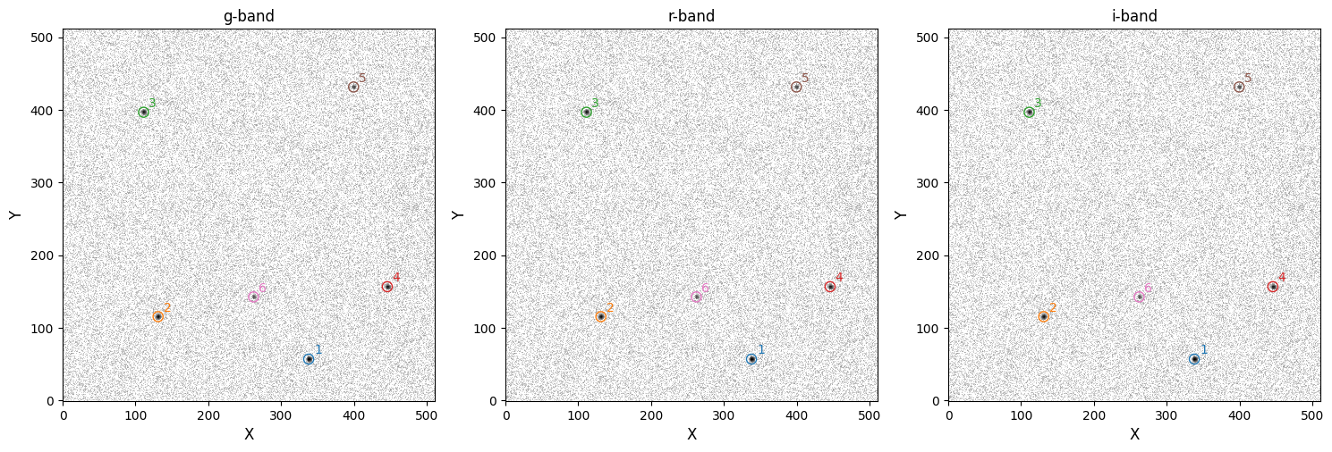
Unsurprisingly, the default source finder has also identified all six sources. Admittedly, this rather simple example does a poor job of demonstrating why defining a custom source finder may be useful, but hopefully it is clear how custom source finders can be implemented. For more information on defining custom source finders, I again refer to the excellent photutils documentation: https://photutils.readthedocs.io/en/stable/user_guide/segmentation.html. Note that opticam requires that
source finder routines return an astropy.table.QTable instance when called.
That concludes the source finder tutorial for opticam!